Posted by Zach Carter

Landscape connectivity (also known as ecological connectivity or landscape permeability) is the degree to which a landscape facilitates or impedes wildlife movement. Understanding landscape connectivity has become a major conservation priority for ecological managers because it can be used to protect and restore important ecological processes; such examples include: the promotion of gene flow/dispersal, creation of risk assessments to characterise the likelihood of invasive species dispersal, and quantification of habitat fragmentation throughout peri-urban regions.

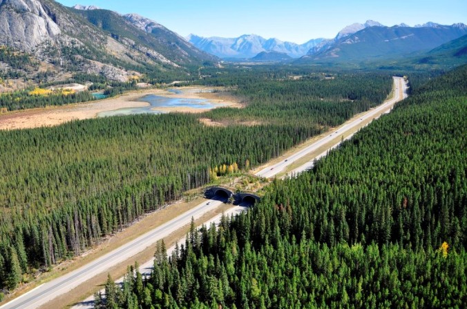An example of landscape connectivity in practice: a conservation corridor that traverses the Trans-Canada Highway in Banff National Park to facilitate large mammal movement (image: https://conservationcorridor.org/2012/10/banff-national-park/)

Most commonly, spatially explicit connectivity models use resistance surfaces to represent landscape features. This is a graph-theoretic technique that reflects movement, represented as a pixel value in a grid within a geographic information system. Connectivity models ultimately use resistance surfaces to calculate the ecological cost associated with movement through a landscape between two termini (starting/ending points). It is assumed that the organism of interest will travel in such a way so as to minimise incurred costs. Accurate representation of these movements can then be used to make informed management decisions based on desired outcomes.

Two common models used for calculating ecological distance include the cost distance and current flow methodologies. These methods propose antithetic assumptions regarding the organism(s) emigration trajectory, where the cost distance model assumes the organism has perfect knowledge of the landscape and will, therefore, choose a path that minimises cumulative ecological costs, and the current flow model which treats the landscape as an electrical circuit and assumes the organism has no prior knowledge of the landscape whatsoever. Often these methods cannot elucidate an organism’s true understanding of the landscape and, as such, are used in conjunction to create a more complete picture.

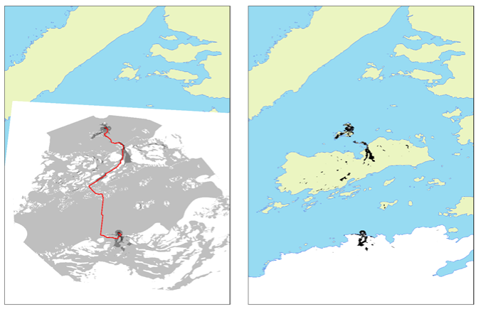An example cost distance (fig. A, least-cost path) and current flow (fig. B, probabilistic movement) output for a generalised mammalian disperser as it emigrates from the New Zealand mainland to an offshore island in Fiordland. The red coloured least-cost path (fig. A) represents the path of least resistance as the organism emigrates. The dark coloured areas (fig. B) represent areas of probabilistic movement from an emigrating organism (source: Z Carter).

Current flow has gained much attention recently for use in connectivity modelling because it considers probabilistic movement across all possible paths within a landscape. If maximising connectivity is the desired ecological outcome (e.g. reducing habitat fragmentation), then calculating current flow between two termini within a landscape is a good model to follow (see fig. B above). On the other hand, if the desired ecological outcome is to reduce organism dispersal (e.g. prevent the spread of invasive species) calculating the least-cost path between termini may be a good modelling option because it often overestimates connectivity. In this instance it would be better to overestimate connectivity than to under estimate it in order to produce informative ecological recommendations regarding the potential spread of a pest species.

For more reading I recommend the following publications:

Etherington, T. R. (2015). “Geographical isolation and invasion ecology.” Progress in Physical Geography 39(6): 697-710.

McRae, B. H. and P. Beier (2007). “Circuit theory predicts gene flow in plant and animal populations.” Proceedings of the National Academy of Sciences 104(50): 19885-19890.

Wade, A. A., et al. (2015). “Resistance-surface-based wildlife conservation connectivity modeling: Summary of efforts in the United States and guide for practitioners.” Gen. Tech. Rep. RMRS-GTR-333. Fort Collins, CO: US Department of Agriculture, Forest Service, Rocky Mountain Research Station. 93 p. 333.

 

Zach Carter is PhD candidate in the School of Biological Sciences at the University of Auckland. His research focuses on developing prioritisation models to assist eradication efforts for the Predator Free 2050 Programme. He is supervised by James Russell and George Perry.